domingo, 2 de septiembre de 2018

MultiLabel and Multiclass Datasets

From time to time in our day-to-day work as data analysts we find strange things, things that can give us a headache, think about  when we study about one classifier algorithm in particular is with simple dataset, where everything goes well, but when we collect the data in our work, Oh surprise! things are not so easy.

Recently, I came across the following problem, I had a dataset from which I had to predict its class, this class was not binary, that is, it was a set of categories, until here everything normal, but, later I noticed  that in fact the dataset not only have one class but three and none of them were binary, well, well, I found a dataset in the UCI repository that explain this problem better. Click to download here.

Basically the dataset contains 22 numerical fields that represent measurements of the sound that some species of frogs do, this dataset has three categories to classify: Families, Genus and Species, each of these, in turn, are multi-classes and its data are:


Families
  • Bufonidae
  • Dendrobatidae
  • Hylidae
  • Leptodactylidae
Genus
  • Adenomera
  • Ameerega
  • Dendropsophus
  • Hypsiboas
  • Leptodactylus
  • Osteocephalus
  • Rhinella
  • Scinax
Species
  • AdenomeraAndre
  • AdenomeraHylaedact
  • Ameeregatrivittata
  • HylaMinuta
  • HypsiboasCinerascens
  • HypsiboasCordobae
  • LeptodactylusFuscus
  • OsteocephalusOopha
  • Rhinellagranulosa
  • ScinaxRuber

And this is where things become interesting, for the same entry we will have three labels, to say: familie, genus and Species which we will have to classify, and each of these labels contain several categories, so how do we work with these datasets?

In this post I will explain step by step how to work with these data sets, I will use the python language for practicality, however, I will explain how this algorithms works, so they can be implemented in the language of your preference.

First we import the libraries that we will use:


Now, we will create a function that will receive a classifier 'x', training data , testing data and we will return its performance


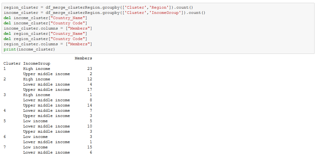
Now we will load and study our dataset (for those who do not know python, the .head () method prints the first 5 rows)


As we can see our data set consists of 7195 rows and 26 columns, of which 3 of them are our labels and the others are our data, all of them numerical, we can see that we do not have to do much about cleaning it, in fact, only I will convert the columns classes into categories to improve the performance a bit.


Well, the next step will be to convert each class into a binary column so that the algorithms can work


The same with the others two classes


Concat the dataframes


Let's separate the original dataframe into two dataframes, that is, one that represents the data and another the classes


Now we generate the training and testing data sets


Now what ?, well, we can not use any algorithm here because it failed miserably, since we have a problem of multilabel, that is, we have to classify here three classes instead of one, let's see an example of how any algorithm would fail


Then what do we do? , well we have three ways to deal with these kind of problems:

  1. - Binary Relevance
  2. - Classifier Chains
  3. - Label Powerset

Binary Relevance:
    This is the divide and conquer, basically it takes each possible class individually and classify it, then concatenate everything and get the result:

Original:


Transforms it into:


Classifier Chains
    This technique first takes only one class column and classifies it, then it takes another class column to classify it but the first will be part of the data, then it will take a third and the first two will be part of the data, ufff, the follow image shows better this process.

Original :


Transforms it into:


The data shaded in yellow are what we would use to classify our class

Label Powerset
    In my opinion the most simple to understand, here we try to label the different conditions in which the classes are generated and we create new classes
Original :


Transforms it into:


This method is the simplest, however, it is worth mentioning that we would need to have all possible combinations to generate all possible classes


Which method is better? Well, sincerely it is better to experiment all the cases to see which one fits our problem, for python we have that the skmultilearn.problem_transform library gives us these methods.


As we observed, at least for this dataset, the techniques that fits better were Chain and Label PowerSet


The complete code can be downloaded  here


jueves, 9 de agosto de 2018

Life Expectancy and Fertility Data Analyst

Is this chapter I analyze the relations between fertility, life expectancy and incomes in the world, I hope you find some interesting tips about how to analyze this kinds of data.

The original dataset is here.

Was necessary to cleaned the data and working with it previously for this analysis, all of the full code is here.

The libraries that I used were:


 We have 5 datasets :

  • Clean_life_expectancy : The provided dataset for life expectancy, cleaned and updated
  • Clean_life_expectancy_Melt : Contains the same info that clean_life_expectancy but with the years columns melting into rows
  • Clean_fertility : The provided dataset for Fertility, cleaned and updated
  • Clean_fertility_Melt : Contains the same info that Clean_fertility but with the years columns melting into rows
  • metadata : Special dataset that contains information that link the country with regions an incomes types

Quick Inspection of the datasets


Merging life_expectancy, fertility and metadata datasets


By region and income

Grouping life and fertility by its median


Verifying Life expectancy over the years


As we noticed the life expectancy are incremental with the time


Verifying Fertility over the years


Fertility is decrementing over the years , this suggest a negative correlation with life expectancy


Verifying the relation between life expectancy and fertility over the years


This confirms the idea that life expectancy and fertility are negative correlated


Verifying if the correlation is negative in all the regions

Obtaining all the regions


Displaying the life expectancy and fertility over the years by region, also showing the correlation by region


As we can see the life expectancy- fertility relation is stable from 20-60 years but passing this threshold, the fertility starts an aggressive decrement, we could check this specially in North America and Europe


Verifying if the correlation is negative with incomes types

Obtaining all the incomes types


Displaying the life expectancy and fertility over the years by incomes types, also showing the correlation by incomes


As we can see the relations between life expectancy and fertility with the incomes types keeps the same behavior like the regions. Here we can noticed that when the income increase the life expectancy increase too and  fertility decrement, again with the threshold of 60 years


Verifying Central Tendency measures by regions


Apparently the most stable region is North America, in the opposite, Asia and Africa suffers by outliers,this could be explain because some countries of this regions are rich and others poor, for example in Africa the differences between South Africa and Somalia are too bigger


Verifying which group(region or income) affect more the relation fertility-life expectancy


Creating a 7 centroids knn cluster (simulating the 7 regions)


Creating a 4 centroids knn cluster (simulating the 4 incomes)


The cluster that obtains a better inertia was the 7 centroid, now we create a hierarchical cluster and determine which distance could provide us similar number of clusters


As we can see with a distance of 9 we have been able to obtain the exact number of desired clusters (7)


Now is time to analyze the information provided by the hierarchical clustering

The next table shows the joining info between the hierarchical clustering and the data provided by the metadata


Grouping the info by income


Grouping the info by Region


Interpretations :

  • We can group the cluster 6 and 7 into one because they are affected in the same manner by the region and the income (Sub-Saharan Africa, South Asia)(Low income,Lower middle income).
  • The clusters 1 and 4 explain better its fertility-life relation for its incomes that for its regions.
  • Both, regions and incomes can explain in certain way the relation fertility - life expectancy, this is possible because some regions has a clearly determine kind of income, for example the mayority of the countries of africa has low incomes in comparision with europe
  • When the income increase, the fertility suffer a decrease and the life expectancy increase
  • When the income decrease, the fertility suffer an increment and the life expectancy decrease
  • Based of this results apparently is more important the incomes , that is to say, the relation between fertility-life expectancy by region is just explained by the incomes of the region

Finally I show the top 20 countries ordered by life expectancy and fertility (here the data was normalized)

By Max Agrupation


Plotting life expectancy and fertility into one single dimension


The countries displaying in the graph above will have the most establish growing in the future (which not mean that will have the most population)


In the other side the countries showing above will have apparently a negative growing in the future.


The chart below shows the countries that are located in the 75% percentile, this location means that this countries will have a better growing population because they combines a good fertility rate with a high life expectancy. Notice the case of France , this country has a high life expectancy (between 75-80 years) but its fertility technically does not have variation over the years and keeping in a good rate up to 2


Here the same data but with life expectancy and fertility normalize


Creating a process that tries to determine under the same conditions which country will have more population in 50 years. Approximately 26.3% of the global population is aged under 15, while 65.9% is aged 15–64 and 7.9% is aged 65 or over.[67] The median age of the world's population was estimated to be 29.7 years in 2014,[69] and is expected to rise to 37.9 years by 2050 


The results of the last exercise were just for fun, because exits a lot of extra factors that is necessary to consider for this, but at least we can have a perspective.


Bibliography